Nyquist Plots

Principle of the Argument

Consider a simple closed contour $C$$\large C$ and a transfer function $H(s)$$\large H(s)$.

Then, $H(C)$$\large H(C)$ will encircle the origin in a clockwise direction $Z-P$$\large Z - P$ times, where

• $Z=$$\large Z =$ number of zeros of $H(s)$$\large H(s)$ inside $C$$\large C$
• $P=$$\large P =$ number of poles of $H(s)$$\large H(s)$ inside $C$$\large C$

Assumption: the contour $C$$\large C$ does not pass through any poles or zeros.

Definition

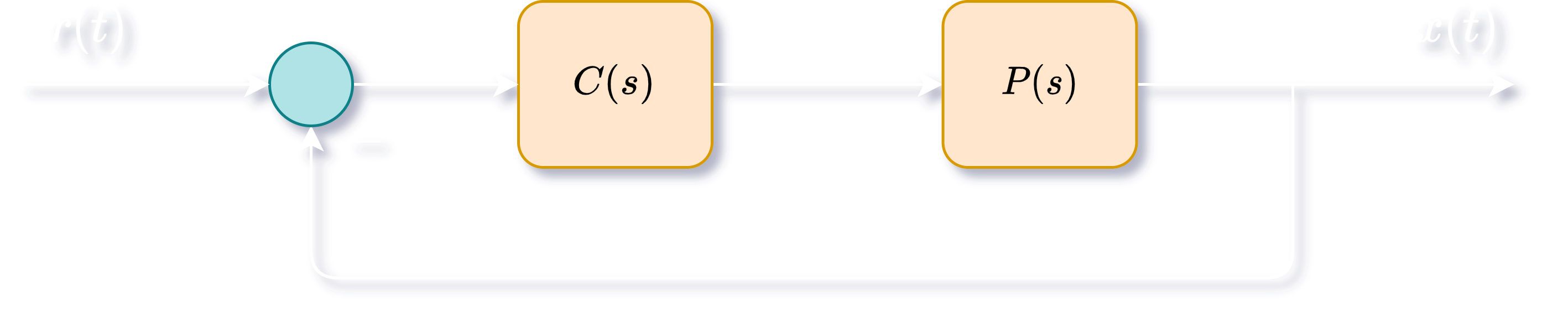
Consider a unity feedback system with reference signal $r(t)$$r(t)$, output signal $y(t)$$y(t)$, plant $P(s)$$P(s)$ and controller $C(s)$$C(s)$.

If we define $L(s)$$L(s)$ such that,

Then,

where the closed loop poles are solutions to $1+L(s)=0$$\large 1 + L(s) = 0$.

Define $H(s)=1+L(s)$$\large H(s) = 1 + L(s)$. Letting $L(s)=\frac{N(s)}{D(s)}$$\large L(s) = \frac{N(s)}{D(s)}$:

This shows that poles of $H(s)$$\large H(s)$ are poles of $L(s)$$\large L(s)$ (open-loop poles) and zeros of $H(s)$$\large H(s)$ are poles of $T_{ry}(s)$$\large T_{ry}(s)$ (closed-loop poles)

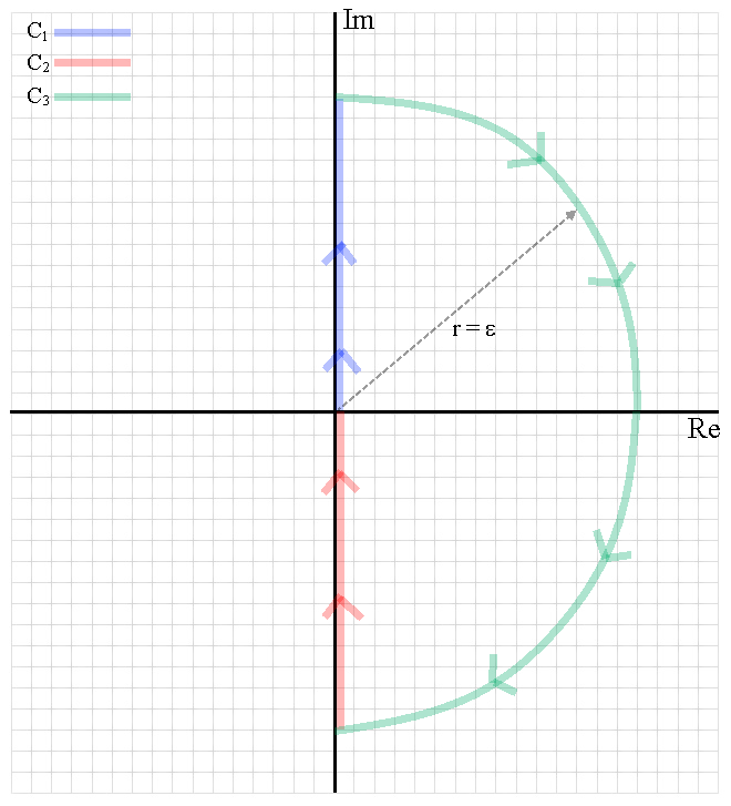
Define a contour C such that:

1. $C_1$$\large C_1$: all points $s=j\omega$$\large s = j\omega$ as $\omega$$\large \omega$ ranges from $0$$\large 0$ to $\mathrm{\infty }$$\large \infty$
2. $C_2$$\large C_2$: all points $s=-j\omega$$\large s = -j\omega$ as $\omega$$\large \omega$ ranges from $\mathrm{\infty }$$\large \infty$ to $0$$\large 0$
3. $C_3$$\large C_3$: semicircle of infinite radius, $s=ϵe^{j\theta }$$\large s = \epsilon e^{j \theta}$, where $ϵ\to \mathrm{\infty }$$\large \epsilon \to \infty$, and $\theta$$\large \theta$ goes from ${90}^{\circ }$$\large 90^{\circ}$ to $-{90}^{\circ }$$\large -90^{\circ}$

$H(C)$$\large H(C)$ is called the Nyquist plot of $H(C)$$\large H(C)$.

Principle of the Argument:

where

• $N=$$\large N =$ number of times the Nyquist plot encircles the origin
• $Z=$$\large Z =$ number of zeros of $H(s)$$\large H(s)$ enclosed by $C$$\large C$, i.e., number of closed-loop poles in RHP
• $P=$$\large P =$ number of poles of $H(s)$$\large H(s)$ enclosed by $C$$\large C$, i.e., number of open-loop poles in RHP

Nyquist plot can also be generated for $L(s)$$\large L(s)$, where $N=$$\large N =$ number of times the Nyquist plot encircles $s=-1$$\large s = -1$ (since $H(s)=1+L(s)$$\large H(s) = 1 + L(s)$)

Drawing Nyquist Plots

Contour $C_1$$C_1$

Contour $C_1$$\large C_1$ consists of points $s=j\omega$$\large s = j \omega$ where $\omega$$\large \omega$ ranges from $0$$\large 0$ to $\mathrm{\infty }$$\large \infty$. Therefore, each point on $L(C_1)$$\large L(C_1)$ is just a complex number $L(j\omega )$$\large L(j \omega)$ with magnitude $|L(j\omega )|$$\large |L(j \omega)|$ and phase $\mathrm{\angle }L(j\omega )$$\large \angle L(j \omega)$.

$C_1$$\large C_1$ can be traced out by looking at the variation of the Bode plot of $L(j\omega )$$\large L(j \omega)$.

Contour $C_2$$C_2$

Contour $C_2$$\large C_2$ consists of points $s=-j\omega$$\large s = -j \omega$ where $\omega$$\large \omega$ ranges from $\mathrm{\infty }$$\large \infty$ to $0$$\large 0$. Therefore, each point on $L(C_2)$$\large L(C_2)$ is just a complex number $L(-j\omega )$$\large L(-j \omega)$ with magnitude $|L(-j\omega )|$$\large |L(-j \omega)|$ and phase $\mathrm{\angle }L(-j\omega )$$\large \angle L(-j \omega)$. In other words, it is the complex conjugate of $L(-j\omega )$$\large L(-j \omega)$.

$L(C_2)$$\large L(C_2)$ is the mirror of $L(C_1)$$\large L(C_1)$ about the real axis.

Contour $C_3$$C_3$

Contour $C_3$$\large C_3$ consists of points in the semicircle $s=ϵe^{j\theta }$$\large s = \epsilon e^{j \theta}$, where $ϵ\to \mathrm{\infty }$$\large \epsilon \to \infty$, and $\theta$$\large \theta$ goes from ${90}^{\circ }$$\large 90^{\circ}$ to $-{90}^{\circ }$$\large -90^{\circ}$. $L(C_3)$$\large L(C_3)$ contains points of the form $L(ϵe^{j\theta })$$\large L(\epsilon e^{j \theta})$. Since $ϵ$$\large \epsilon$ is infinite, the term in $L(ϵe^{j\theta })$$\large L(\epsilon e^{j \theta})$ with the highest power of $ϵ$$\large \epsilon$ will dominate.

If $L(s)$$\large L(s)$ is strictly proper, $L(C_3)=0$$\large L(C_3) = 0$.

If $L(s)$$\large L(s)$ is proper, (but not strictly proper), $L(C_3)$$\large L(C_3)$ is a constant

Stability Margins

We can determine the stability margins using the Nyquist plot.

Gain Margin is the gain required to make the Nyquist plot intersect the negative real axis at -1. In other words, the length from the origin to the point where the Nyquist plot intersects the negative real axis is $\frac{1}{GM}$$\large \frac{1}{GM}$.

Phase Margin is the angle between the point where the Nyquist plot enters the unit circle and the -1 point about the origin.